Subscribe to my newsletter
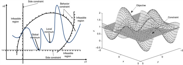
In Operations Research domain, there are variety of Constrained Optimzation algorithms. For most of them, many solvers have developed python APIs within libraries like Pulp, Pyomo, Scipy, Gurobi.
I found couple of good articles summarizing the differences among these libraries in terms of building the problem and syntaxes:
- https://medium.com/analytics-vidhya/optimization-modelling-in-python-scipy-pulp-and-pyomo-d392376109f4
- https://medium.com/opex-analytics/optimization-modeling-in-python-pulp-gurobi-and-cplex-83a62129807a
What this post is about
After covering few articles, I realized PuLP and Gurobi are few among powerful solvers with python API. (Also, Scipy has more integration capabilities with Python). I wanted to try out these 2 solvers with some problems over the internet.
Installation was easy for both of them. PuLP is open source and easy to install, also can be extended for variety of solvers. Gurobipy installation comes with a trial period.
I will cover 3 problems:
- Blending problem using PuLP:
- Unbalanced Transportation Problem using puLP
- Factory planning - Generic cosntrained Optimzation
1. Blending Problem
I found the problem from Stanford coursework here solved using inbuilt matlab solver. I went through PuLP documentation to understand the formalization of problem, how to add variables, constraints, define objective, and solve. PuLP documentation was quite good. I follwed this page to recreate solution for my problem.
problem:
Formulation involves splitting stock capacity in two parts - used and unused. So the Objective statement will be to maximize the sales along with maximizing the unused stocks.
Formulation for matlab:
Using PuLP and following documentation:
from pulp import *

#define the problem
prob = LpProblem("The blending Problem", LpMaximize)

#define the variables
S1A = LpVariable("UsedStockOneInA", 0, 2000, LpInteger)
S1B = LpVariable("UsedStockOneInB", 0, 2000, LpInteger)

S2A = LpVariable("UsedStockTwoInA", 0, 4000, LpInteger)
S2B = LpVariable("UsedStockTwoInB", 0, 4000, LpInteger)

S3A = LpVariable("UsedStockThreeInA", 0, 4000, LpInteger)
S3B = LpVariable("UsedStockThreeInB", 0, 4000, LpInteger)

S4A = LpVariable("UsedStockFourInA", 0, 5000, LpInteger)
S4B = LpVariable("UsedStockFourInB", 0, 5000, LpInteger)

S5A = LpVariable("UsedStockFiveInA", 0, 3000, LpInteger)
S5B = LpVariable("UsedStockFiveInB", 0, 3000, LpInteger)

US1 = LpVariable("UnusedStockOne", 0, None, LpInteger)
US2 = LpVariable("UnusedStockTwo", 0, None, LpInteger)
US3 = LpVariable("UnusedStockThree", 0, None, LpInteger)
US4 = LpVariable("UnusedStockFour", 0, None, LpInteger)
US5 = LpVariable("UnusedStockFive", 0, None, LpInteger)

FA = LpVariable("FuelBlendA", 0, None, LpInteger)
FB = LpVariable("FuelBlendB", 0, None, LpInteger)

#using prob += first thing should be added is the objective
#Objective here is to maximize the unused stock - first 4 terms and also sales revenue - last 2 terms.
prob += (9*US1) + (12.5*US2) + (12.5*US3) + (27.5*US4) + (27.5*US5) + (37.5*FA) + (28.5*FB), "maximize value of total unused stock and income"

#we can add constrained based on availability of stocks
prob += S1A + S1B + US1 == 2000, "TotalAvailabilityOfStock1"
prob += S2A + S2B + US2 == 4000, "TotalAvailabilityOfStock2"
prob += S3A + S3B + US3 == 4000, "TotalAvailabilityOfStock3"
prob += S4A + S4B + US4 == 5000, "TotalAvailabilityOfStock4"
prob += S5A + S5B + US5 == 3000, "TotalAvailabilityOfStock5"

#quantity constraints
prob += S1A + S2A + S3A + S4A + S5A == FA, "TotalQuantityOfBlendA"
prob += S1B + S2B + S3B + S4B + S5B == FB, "TotalQuantityOfBlendB"

#quality constraints
prob += (70*S1A) + (80*S2A) + (85*S3A) + (90*S4A) + (99*S5A)  >= 93*FA, "QualityOfBlendA"
prob += (70*S1B) + (80*S2B) + (85*S3B) + (90*S4B) + (99*S5B)  >= 85*FB, "QualityOfBlendB"

#define the path for ouput file - optional
prob.writeLP("BlendModel.lp")

#solve
prob.solve()

#status of solver
print("Status:", LpStatus[prob.status])
#output : Status: Optimal

#results for each variable
for v in prob.variables():
    print(v.name, "=", v.varValue)
#output:
FuelBlendA = 2125.0
FuelBlendB = 15875.0
UnusedStockFive = 0.0
UnusedStockFour = 0.0
UnusedStockOne = 0.0
UnusedStockThree = 0.0
UnusedStockTwo = 0.0
UsedStockFiveInA = 710.0
UsedStockFiveInB = 2290.0
UsedStockFourInA = 1413.0
UsedStockFourInB = 3587.0
UsedStockOneInA = 0.0
UsedStockOneInB = 2000.0
UsedStockThreeInA = 1.0
UsedStockThreeInB = 3999.0
UsedStockTwoInA = 1.0
UsedStockTwoInB = 3999.0

#objective function solved
print("Total Income from two blends = ", value(prob.objective))
#output: Total Income from two blends =  532125.0
From the source of the problem, matlab solver also produced the same answer.
2. Unbalanced Transportation Problem
Unbalanced transportation problems are classic supply demand optimization considering route costs. I found a problem here. Transportation problem solving is lot of fun with hand calculation using methods like, VAM, MODI, Northwest Corner Method, Minimum Cost methods.
After going through PuLP documentation, I formulated the problem as:
#supply nodes
warehouses = ['O1', 'O2', 'O3', 'D']

# Creates a dictionary for the number of units of supply for each supply node
supply = {"O1": 70, "O2": 55, "O3": 70, "D": 20} #D is dummy node to balance

# Creates a list of all demand nodes
Destinations = ["D1", "D2", "D3", "D4"]

# Creates a dictionary for the number of units of demand for each demand node
demand = {"D1": 85, "D2": 35, "D3": 50, "D4": 45} #M

# Creates a list of costs of each transportation path
costs = [  # Destinations
    # 1   2   3   4
    [6,  1,  9,  3],  # O1   Supply Nodes
    [11, 5,  2,  8],  # O2
    [10, 12, 4,  7],  # O3
    [0,  0,  0,  0],  # D  route costs for dummy node are zeros
]

# The cost data is made into a dictionary
costs = makeDict([warehouses, Destinations],costs,0)

# Creates the 'prob' variable to contain the problem data
prob = LpProblem("Unbalanced Transportation Problem",LpMinimize)

# Creates a list of tuples containing all the possible routes for transport
Routes = [(w,d) for w in warehouses for d in Destinations]
Routes
#output:
'''
[('O1', 'D1'),
 ('O1', 'D2'),
 ('O1', 'D3'),
 ('O1', 'D4'),
 ('O2', 'D1'),
 ('O2', 'D2'),
 ('O2', 'D3'),
 ('O2', 'D4'),
 ('O3', 'D1'),
 ('O3', 'D2'),
 ('O3', 'D3'),
 ('O3', 'D4'),
 ('D', 'D1'),
 ('D', 'D2'),
 ('D', 'D3'),
 ('D', 'D4')]
'''

# A dictionary called 'Vars' is created to contain the referenced variables(the routes)
vars = LpVariable.dicts("Route",(warehouses, Destinations), 0, None, LpInteger)
vars
#output:
'''
{'O1': {'D1': Route_O1_D1,
  'D2': Route_O1_D2,
  'D3': Route_O1_D3,
  'D4': Route_O1_D4},
 'O2': {'D1': Route_O2_D1,
  'D2': Route_O2_D2,
  'D3': Route_O2_D3,
  'D4': Route_O2_D4},
 'O3': {'D1': Route_O3_D1,
  'D2': Route_O3_D2,
  'D3': Route_O3_D3,
  'D4': Route_O3_D4},
 'D': {'D1': Route_D_D1, 'D2': Route_D_D2, 'D3': Route_D_D3, 'D4': Route_D_D4}}
'''

# The objective function is added to 'prob' first
prob += lpSum([vars[w][d]*costs[w][d] for (w,d) in Routes]), "Sum_of_Transporting_Costs"

# The supply maximum constraints are added to prob for each supply node (warehouse)
for w in warehouses:
    prob += lpSum([vars[w][d] for d in Destinations]) <= supply[w], "Sum_of_Products_out_of_Warehouse_%s"%w

# The demand minimum constraints are added to prob for each demand node (bar)
for d in Destinations:
    prob += lpSum([vars[w][d] for w in warehouses]) >= demand[d], "Sum_of_Products_into_Destinations%s"%d

# The problem data is written to an .lp file
prob.writeLP("UnbalancedTransportationProblem.lp")

# The problem is solved using PuLP's choice of Solver
prob.solve()

# The status of the solution is printed to the screen
print("Status:", LpStatus[prob.status])
#output: Status: Optimal

# Each of the variables is printed with it's resolved optimum value
for v in prob.variables():
    print(v.name, "=", v.varValue)
#output
'''
Route_D_D1 = 20.0
Route_D_D2 = 0.0
Route_D_D3 = 0.0
Route_D_D4 = 0.0
Route_O1_D1 = 0.0
Route_O1_D2 = 30.0
Route_O1_D3 = 0.0
Route_O1_D4 = 40.0
Route_O2_D1 = 0.0
Route_O2_D2 = 5.0
Route_O2_D3 = 50.0
Route_O2_D4 = 0.0
Route_O3_D1 = 65.0
Route_O3_D2 = 0.0
Route_O3_D3 = 0.0
Route_O3_D4 = 5.0
'''

# The optimised objective function value is printed to the screen
print("Total Cost of Transportation = ", value(prob.objective))
#output: Total Cost of Transportation =  960.0
Answer matches the solution on the source.
3. Factory planning - Generic cosntrained Optimzation
Gurobipy has a good documentation on a variety of forulations for complex problems with examples in python. I recreated custom version of factory planning problem as further:
problem
A factory makes six products (P1 to P6). Profit margin on each product is: “P1”:10, “P2”:15, “P3”:8, “P4”:6, “P5”:6, “P6”:10
Workshop is equiped with: 3 Inspectiontables 2 Multiaxial CNC1s 3 CoAxial CNC2s 2 Grinders 1 Planers 4 Reassembly areas
The factory is functional 5 days a week using two eight-hour shifts per day. It may be assumed that each month consists of 4 weeks. There are no production sequencing conditions for the simplicity.
At the start of January, there is no product inventory.
Up to 200 units of each product may be stored in inventory.
Inventory cost is $0.20 per unit per month.
By the end of May, to prepare for the memorial day, there should be 40 units of each product in inventory.
Let’s start with formulation:
import numpy as np
import pandas as pd

import gurobipy as gp
from gurobipy import GRB

products = ["P1", "P2", "P3", "P4", "P5", "P6"]
machines = ["inspectionTable", "CNC1", "CNC2", "grinder", "planer", "reassemblyArea"]
months = ["Jan", "Feb", "Mar", "Apr", "May"]

profit = {"P1":10, "P2":15, "P3":8, "P4":6, "P5":6, "P6":10}

time_req = {
    "inspectionTable": {"P1": 0.5, "P2": 0.7, "P3": 0.8, "P4": 0.6, "P5": 0.3, "P6": 0.2},
    "CNC1": {"P1": 0.3, "P3": 0.3, "P5": 0.6},
    "CNC2": {"P1": 0.2, "P5": 0.8, "P6": 0.6},
    "grinder": {"P1": 0.05,"P2": 0.03,"P3": 0.07, "P5": 0.1, "P6": 0.08},
    "planer": {"P1": 0.5, "P2": 0.2, "P4": 0.3, "P6": 0.6},
    "reassemblyArea" : {"P1": 0.3, "P2": 0.7, "P3": 0.3, "P4": 0.6, "P5": 0.3, "P6": 0.2}
}


# number of machines down
down = {("Jan","inspectionTable"): 1, ("Jan","ReassemblyArea"): 2,
        ("Feb", "CNC2"): 2,
        ("Mar", "grinder"): 1,
        ("Apr", "CNC1"): 1,
        ("May", "inspectionTable"): 1, ("May", "CNC1"): 1}

# number of each machine available
installed = {"inspectionTable":3, "CNC1":2, "CNC2":3, "grinder":2, "planer":1, "reassemblyArea":4}

# market limitation of sells
max_sales = {
    ("Jan", "P1") : 500,
    ("Jan", "P2") : 500,
    ("Jan", "P3") : 1000,
    ("Jan", "P4") : 400,
    ("Jan", "P5") : 200,
    ("Jan", "P6") : 500,

    ("Feb", "P1") : 300,
    ("Feb", "P2") : 600,
    ("Feb", "P3") : 0,
    ("Feb", "P4") : 0,
    ("Feb", "P5") : 500,
    ("Feb", "P6") : 400,

    ("Mar", "P1") : 600,
    ("Mar", "P2") : 300,
    ("Mar", "P3") : 200,
    ("Mar", "P4") : 0,
    ("Mar", "P5") : 700,
    ("Mar", "P6") : 300,

    ("Apr", "P1") : 200,
    ("Apr", "P2") : 100,
    ("Apr", "P3") : 200,
    ("Apr", "P4") : 500,
    ("Apr", "P5") : 200,
    ("Apr", "P6") : 450,

    ("May", "P1") : 100,
    ("May", "P2") : 100,
    ("May", "P3") : 300,
    ("May", "P4") : 0,
    ("May", "P5") : 400,
    ("May", "P6") : 300
}

max_inventory = 200
holding_cost = 0.2
store_target = 40
hours_per_month = 2*8*20

factory = gp.Model('Factory Planning')

make = factory.addVars(months, products, name="Make") # quantity manufactured
store = factory.addVars(months, products, ub=max_inventory, name="Store") # quantity stored
sell = factory.addVars(months, products, ub=max_sales, name="Sell") # quantity sold

#machine capacity constraint
MachineCap = factory.addConstrs((gp.quicksum(time_req[machine][product] * make[month, product]
                             for product in time_req[machine])
                    <= hours_per_month * (installed[machine] - down.get((month, machine), 0))
                    for machine in machines for month in months),
                   name = "Capacity")


#adding inventory balances
Balance0 = factory.addConstrs((make[months[0], product] == sell[months[0], product]
                  + store[months[0], product] for product in products), name="Initial_Balance")

Balance = factory.addConstrs((store[months[months.index(month) -1], product] +
                make[month, product] == sell[month, product] + store[month, product]
                for product in products for month in months
                if month != months[0]), name="Balance")

#constraint for end target balance of 40 units
TargetInv = factory.addConstrs((store[months[-1], product] == store_target for product in products),  name="End_Balance")

#defining the objective function
obj = gp.quicksum(profit[product] * sell[month, product] -  holding_cost * store[month, product]
               for month in months for product in products)

factory.setObjective(obj, GRB.MAXIMIZE)

#solving
factory.optimize()
#output:
'''
Gurobi Optimizer version 9.1.2 build v9.1.2rc0 (win64)
Thread count: 4 physical cores, 8 logical processors, using up to 8 threads
Optimize a model with 66 rows, 90 columns and 255 nonzeros
Model fingerprint: 0xf68c8638
Coefficient statistics:
  Matrix range     [3e-02, 1e+00]
  Objective range  [2e-01, 2e+01]
  Bounds range     [1e+02, 1e+03]
  RHS range        [4e+01, 1e+03]
Presolve removed 28 rows and 18 columns
Presolve time: 0.01s
Presolved: 38 rows, 72 columns, 171 nonzeros

Iteration    Objective       Primal Inf.    Dual Inf.      Time
       0    9.4352000e+04   1.385400e+03   0.000000e+00      0s
      16    6.5121333e+04   0.000000e+00   0.000000e+00      0s

Solved in 16 iterations and 0.01 seconds
Optimal objective  6.512133333e+04
'''

#optional to create result file
factory.write("factory-planning-1-output.sol")
Analyzing output using same code as on Gurobi documentaiton page
#for sells plan
rows = months.copy()
columns = products.copy()
sell_plan = pd.DataFrame(columns=columns, index=rows, data=0.0)

for month, product in sell.keys():
    if (abs(sell[month, product].x) > 1e-6):
        sell_plan.loc[month, product] = np.round(sell[month, product].x, 1)
sell_plan
#output:
'''
    P1   P2    P3   P4  P5  P6
Jan	0.0	500.0	130.2	0.0	200.0	366.7
Feb	300.0	600.0	0.0	0.0	500.0	0.0
Mar	600.0	300.0	200.0	0.0	700.0	0.0
Apr	200.0	100.0	200.0	500.0	200.0	100.0
May	100.0	100.0	300.0	0.0	400.0	300.0
'''

#production plan
rows = months.copy()
columns = products.copy()
make_plan = pd.DataFrame(columns=columns, index=rows, data=0.0)

for month, product in make.keys():
    if (abs(make[month, product].x) > 1e-6):
        make_plan.loc[month, product] = np.round(make[month, product].x, 1)
make_plan
#output
'''
    p1  p2    p3    p4  p5    p6
Jan	0.0	500.0	130.2	0.0	375.0	366.7
Feb	300.0	800.0	93.3	33.3	325.0	0.0
Mar	600.0	100.0	106.7	0.0	713.3	0.0
Apr	200.0	100.0	200.0	466.7	333.3	100.0
May	140.0	140.0	340.0	40.0	293.3	340.0
'''

#inventory plan
rows = months.copy()
columns = products.copy()
store_plan = pd.DataFrame(columns=columns, index=rows, data=0.0)

for month, product in store.keys():
    if (abs(store[month, product].x) > 1e-6):
        store_plan.loc[month, product] = np.round(store[month, product].x, 1)
store_plan
#output:
'''
   p1  p2    p3    p4  p5    p6
Jan	0.0	0.0	0.0	0.0	175.0	0.0
Feb	0.0	200.0	93.3	33.3	0.0	0.0
Mar	0.0	0.0	0.0	33.3	13.3	0.0
Apr	0.0	0.0	0.0	0.0	146.7	0.0
May	40.0	40.0	40.0	40.0	40.0	40.0
'''
#notice the constraint of end inventory for each product being 40 is satisfied.